import arviz as az
import numpy as np

import pymc as pm

print(f"Running on PyMC v{pm.__version__}")

Running on PyMC v5.27.0+57.g9ffda82e0.dirty

az.style.use("arviz-variat")

Model comparison

To demonstrate the use of model comparison criteria in PyMC, we implement the 8 schools example from Section 5.5 of Gelman et al (2003), which attempts to infer the effects of coaching on SAT scores of students from 8 schools. Below, we fit a pooled model, which assumes a single fixed effect across all schools, and a hierarchical model that allows for a random effect that partially pools the data.

The data include the observed treatment effects (y) and associated standard deviations (sigma) in the 8 schools.

y = np.array([28, 8, -3, 7, -1, 1, 18, 12])
sigma = np.array([15, 10, 16, 11, 9, 11, 10, 18])
J = len(y)

Pooled model

with pm.Model() as pooled:
    # Latent pooled effect size
    mu = pm.Normal("mu", 0, sigma=1e6)

    obs = pm.Normal("obs", mu, sigma=sigma, observed=y)

    trace_p = pm.sample(2000)

Initializing NUTS using jitter+adapt_diag...
Multiprocess sampling (4 chains in 4 jobs)
NUTS: [mu]

Sampling 4 chains for 1_000 tune and 2_000 draw iterations (4_000 + 8_000 draws total) took 2 seconds.

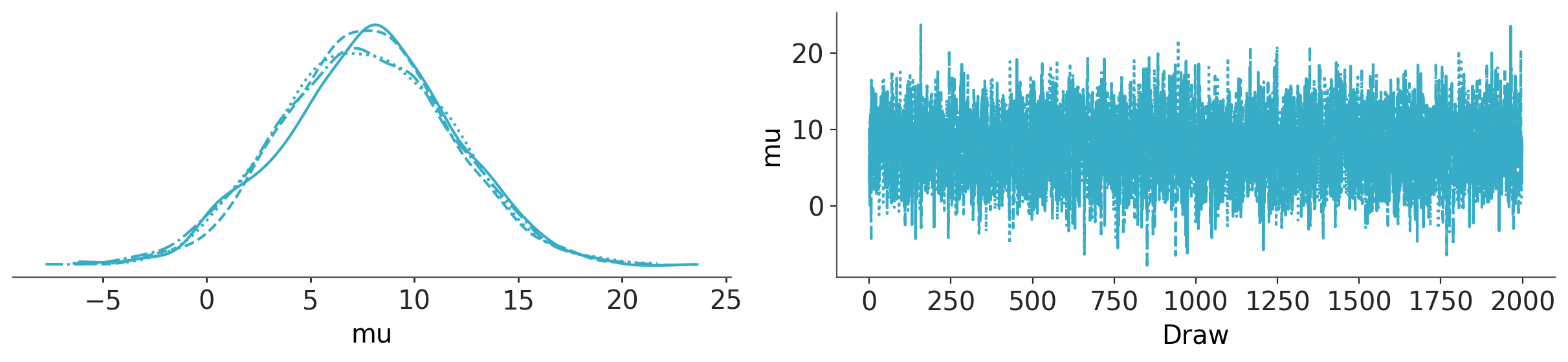
az.plot_trace_dist(trace_p);

Hierarchical model

with pm.Model() as hierarchical:
    eta = pm.Normal("eta", 0, 1, shape=J)
    # Hierarchical mean and SD
    mu = pm.Normal("mu", 0, sigma=10)
    tau = pm.HalfNormal("tau", 10)

    # Non-centered parameterization of random effect
    theta = pm.Deterministic("theta", mu + tau * eta)

    obs = pm.Normal("obs", theta, sigma=sigma, observed=y)

    trace_h = pm.sample(2000, target_accept=0.9)

Initializing NUTS using jitter+adapt_diag...
Multiprocess sampling (4 chains in 4 jobs)
NUTS: [eta, mu, tau]

Sampling 4 chains for 1_000 tune and 2_000 draw iterations (4_000 + 8_000 draws total) took 7 seconds.

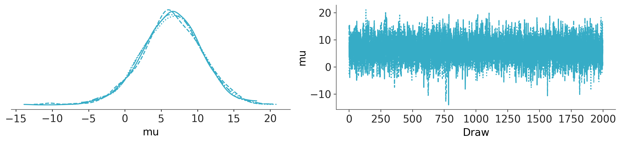
az.plot_trace_dist(trace_h, var_names="mu");

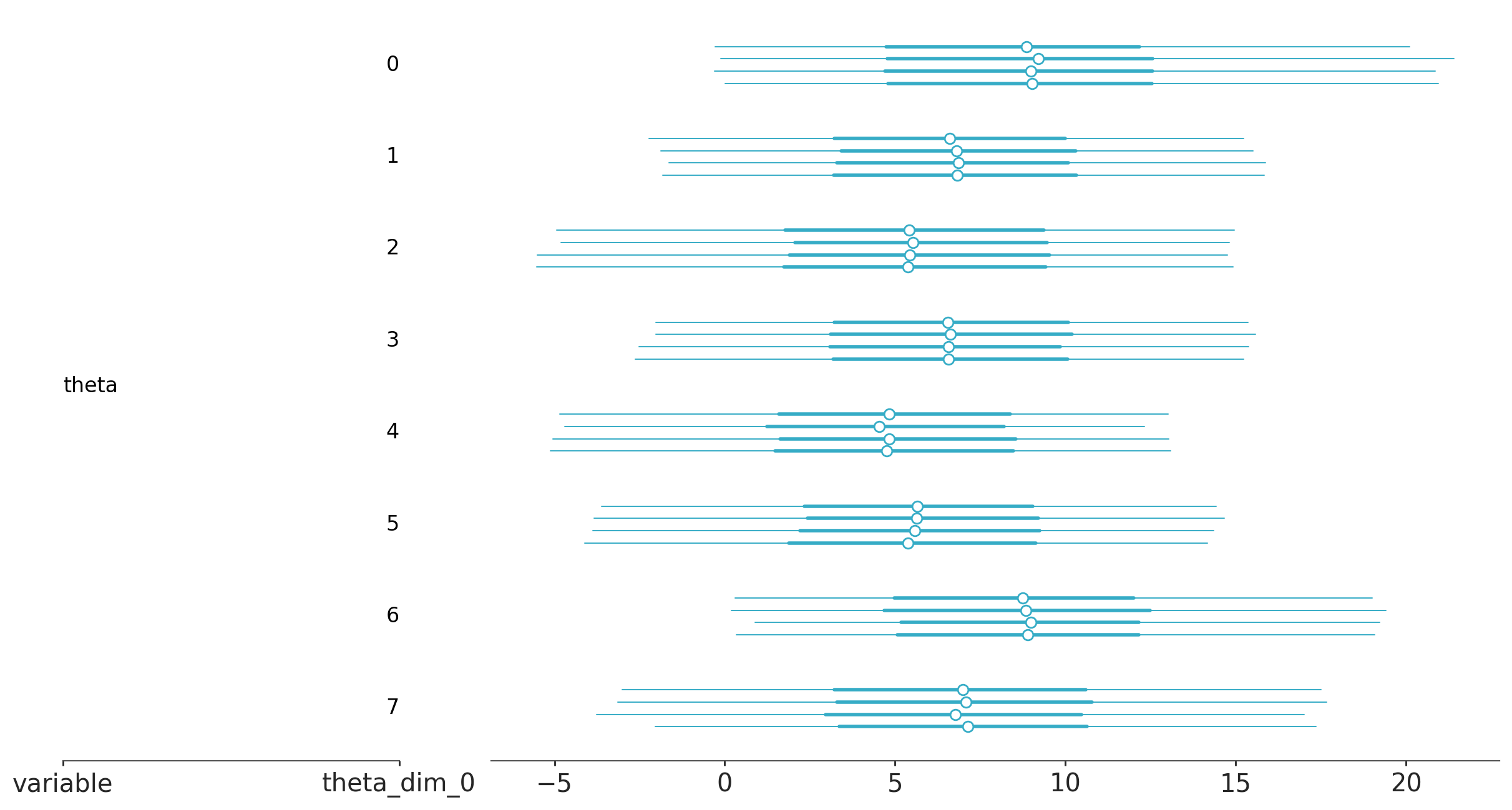
az.plot_forest(trace_h, var_names="theta");

Leave-one-out Cross-validation (LOO-CV)

The expected log pointwise predictive density (ELPD) quantifies how well a model is expected to predict new observations, averaged over data points. This quantity can be estimated in several ways, including cross-validation. In cross-validation, In cross-validation, the data are repeatedly partitioned into training and holdout sets, iteratively fitting the model with the former and evaluating the fit with the holdout data. When each data point is held out once, this is known as leave-one-out cross-validation (LOO-CV). Vehtari et al. (2016) introduced an efficient computation of LOO from MCMC samples (without the need for re-fitting the data). This approximation is based on importance sampling. The importance weights are stabilized using a method known as Pareto-smoothed importance sampling (PSIS), hence the full name PSIS-LOO-CV, but it is commonly referred to as LOO for brevity.

Model log-likelihood

In order to compute LOO, ArviZ needs access to the model elemwise loglikelihood for every posterior sample. We can add it via compute_log_likelihood(). Alternatively we can pass idata_kwargs={"log_likelihood": True} to sample() to have it computed automatically at the end of sampling.

with pooled:
    pm.compute_log_likelihood(trace_p)

pooled_loo = az.loo(trace_p)

pooled_loo

Computed from 8000 posterior samples and 8 observations log-likelihood matrix.

         Estimate       SE
elpd_loo   -30.57     1.11
p_loo        0.68        -
------

Pareto k diagnostic values:
                         Count   Pct.
(-Inf, 0.70]   (good)        8  100.0%
   (0.70, 1]   (bad)         0    0.0%
    (1, Inf)   (very bad)    0    0.0%

with hierarchical:
    pm.compute_log_likelihood(trace_h)

hierarchical_loo = az.loo(trace_h)

hierarchical_loo

Computed from 8000 posterior samples and 8 observations log-likelihood matrix.

         Estimate       SE
elpd_loo   -30.79     1.07
p_loo        1.15        -
------

Pareto k diagnostic values:
                         Count   Pct.
(-Inf, 0.70]   (good)        8  100.0%
   (0.70, 1]   (bad)         0    0.0%
    (1, Inf)   (very bad)    0    0.0%

ArviZ includes two convenience functions to help compare the ELPD for different models. The first of these functions is compare, which uses the PSIS-LOO-CV method to compute the ELPD from a set of traces and models and returns a DataFrame.

df_comp_loo = az.compare({"hierarchical": hierarchical_loo, "pooled": pooled_loo})
df_comp_loo

	rank	elpd	p	elpd_diff	weight	se	dse	warning
pooled	0	-30.57153	0.683161	0.00000	1.0	1.107647	0.000000	False
hierarchical	1	-30.78649	1.149336	0.21496	0.0	1.068123	0.240133	False

We have many columns, so let’s check out their meaning one by one:

0. The index is the names of the models taken from the keys of the dictionary passed to compare(.).

1. rank, the ranking of the models starting from 0 (best model) to the number of models.

2. elpd_loo, the values of the ELPD computed using LOO. The DataFrame is always sorted from best LOO to worst.

3. p_loo, the value of the penalization term. We can roughly think of this value as the estimated effective number of parameters (but do not take that too seriously).

4. elpd_diff, the relative difference between the value of ELPD for the top-ranked model and the value of ELPD for each model. For this reason we will always get a value of 0 for the first model.

5. weight, the weights assigned to each model. These weights can be loosely interpreted as the probability of each model being true (among the compared models) given the data.

6. se, the standard error for the estimated ELPD quantities. The standard error can be useful to assess the uncertainty of the estimates. By default these errors are computed using stacking.

7. dse, the standard errors of the difference between two values of ELPD. The same way that we can compute the standard error for each value of ELPD, we can compute the standard error of the differences between two values of ELPD. Notice that both quantities are not necessarily the same, the reason is that the uncertainty about ELPD is correlated between models. This quantity is always 0 for the top-ranked model.

8. warning, If True the PSIS-LOO-CV method may not be reliable.

9. loo_scale, the scale of the reported values. The default is the log scale as previously mentioned. Other options are deviance – this is the log-score multiplied by -2 (this reverts the order: a lower ELPD will be better) – and negative-log – this is the log-score multiplied by -1 (as with the deviance scale, a lower value is better).

The second convenience function takes the output of compare and produces a summary plot in the style of the one used in the book Statistical Rethinking by Richard McElreath (check also this port of the examples in the book to PyMC).

az.plot_compare(df_comp_loo);

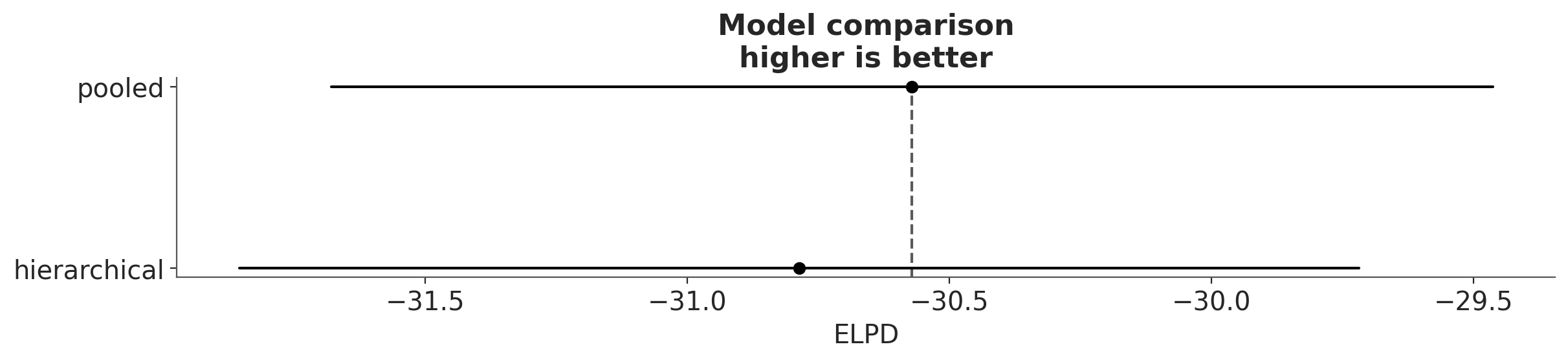
The circles represent the ELPD values and the black error bars associated with them are the values of the standard deviation of the ELPDs.

The value of the highest ELPD, i.e the best estimated model, is also indicated with a vertical dashed grey line to ease comparison with other ELPD values.

For all models except the top-ranked one we also get a triangle indicating the value of the difference of ELPD between that model and the top model and a grey error bar indicating the standard error of the differences between the top-ranked ELPD and ELPD for each model.

Interpretation

Though we might expect the hierarchical model to outperform a complete pooling model, there is little to choose between the models in this case, given that both models gives very similar values of the expected log predictive density (ELPD). This is more clearly appreciated when we take into account the uncertainty (in terms of standard errors).

Reference

Gelman, A., Hwang, J., & Vehtari, A. (2014). Understanding predictive information criteria for Bayesian models. Statistics and Computing, 24(6), 997–1016.

Vehtari, A, Gelman, A, Gabry, J. (2016). Practical Bayesian model evaluation using leave-one-out cross-validation and WAIC. Statistics and Computing

%load_ext watermark

%watermark -n -u -v -iv -w -p xarray,pytensor

Last updated: Sat Feb 14 2026

Python implementation: CPython
Python version       : 3.13.5
IPython version      : 9.3.0

xarray  : 2025.6.1
pytensor: 2.36.1

numpy: 2.2.6
arviz: 1.0.0rc0
pymc : 5.25.1+59.g4ba1d2f1c.dirty

Watermark: 2.5.0